Plot band structure¶

In python environment, band structure can be plotted by calling the mcu.plot_band() function

import mcu
mymcu = mcu.VASP()    # or mymcu = mcu.VASP(path='path-to-vasprun', vaspruns='vasprun')
mymcu.plot_band()

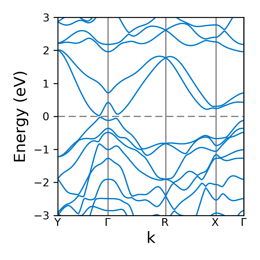
To customize the band, one can modify some of these attributes. For /mcu/example/MoS2, you can run:

import mcu
mymcu = mcu.VASP()
mymcu.plot_band(spin=0, save=True, label='Y-G-R-X-G', fontsize= 9, ylim=(-3,3), figsize=(3,3), dpi=300, format='png')

You should get:

All parameters and their defaults of plot_band function are given below. Most of the parameters are passed to matplotlib functions. So more information can be found in matplotlib docs.

Parameters¶

efermifloat

Default: fermi level from vasprun.xml or OUTCAR
User can shift the Fermi level to a value

spinint

Default: 0
If ISPIN = 1: spin = 0
If ISPIN = 2: spin = 0 (up spin) or 1 (down spin)

labelstr or list

Default: None
For conventional band structure, e.g. label = ‘X-G-Y-L-G’
For hydrib functional band structure, e.g. label = [[‘L’,0.50,0.50,0.50],[‘G’,0.0,0.0,0.00],[‘X’,0.5,0.0,0.50],[‘W’,0.50,0.25,0.75]]

savebool

Default: False
True to save to an image

band_color: list

Default: [‘#007acc’,’#808080’,’#808080’]
Three color codes indice color of band curve, kpoint grid, Fermi level, respectively.
Exp: [‘k’,’#808080’,’r’]
Hex color code can be found here here

figsizetuple or list

Default: De(6,6)
Size of image in inch

fignamestr

Default: ‘BAND’
Name of the image

xlimlist or tuple

Default: None
Limit range for momentum (k) axis. Used when to zoom in a specific range of k with the unit \(Angstrom^{-1}\)

ylimlist or tuple

Default: [-6,6]
Limit range for energy axis in eV

fontsizeint

Default: 18
Font size

dpiint

Default: 600
Resolution of the image

formatstr

Default: ‘png’
Extension of the image

Plot projected band structure¶

In python environment, band structure can be plotted by calling the mcu.plot_band() function

import mcu
mymcu = mcu.VASP()
mymcu.plot_pband()

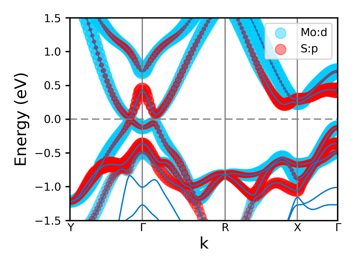
To customize the band, one can modify some of these attributes. For /mcu/example/MoS2, you can run:

import mcu
mymcu = mcu.VASP()
label = 'Y-G-R-X-G'
mymcu.plot_pband(style=2, lm=['Mo:d','S:p'], color=['#00ccff','#ff0000'], alpha=0.4, label=label, fontsize= 9, ylim=(-1.5,1.5),figsize=(4,3),legend=['Mo:d','S:p'],legend_size=1.2, save=True, figname='MoS2_style2', dpi=300)

You should get:

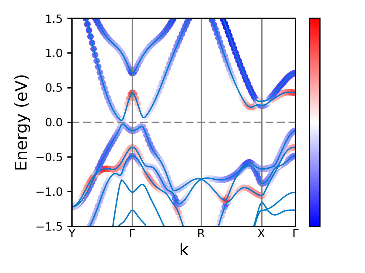
Or for style = 3:

import mcu
mymcu = mcu.VASP()
label = 'Y-G-R-X-G'
mymcu.plot_pband(style=3, lm='pd', label=label, fontsize= 9, scale=0.5, ylim=(-1.5,1.5), figsize=(4,3), save=True, figname='MoS2_style3', dpi=300)

All parameters and their defaults of plot_pband function are given below. Most of the parameters are passed to plot_band function. Some of additional parameters for projected band structure. Most important parameters are style and lm.

Parameters¶

efermifloat

Default: fermi level from vasprun.xml or OUTCAR
User can shift the Fermi level to a value

spinint

Default: 0
If ISPIN = 1: spin = 0
If ISPIN = 2: spin = 0 (Up spin) or 1 (Down spin)

labelstr or a list of str

Default: None
For conventional band structure, e.g. label = ‘X-G-Y-L-G’
For hydrib functional band structure, e.g. label = [[‘L’,0.50,0.50,0.50],[‘G’,0.0,0.0,0.00],[‘X’,0.5,0.0,0.50],[‘W’,0.50,0.25,0.75]]

band_color: list

Default: [‘#007acc’,’#808080’,’#808080’]
Three color codes indice color of band curve, kpoint grid, Fermi level, respectively.
Exp: [‘k’,’#808080’,’r’]
Hex color code can be found here here

styleint

Default: 1
If style = 1: the most flexible style, all atoms are considered. A few examples of lm are:
- Choose one specific orbital: lm = ‘s’ or lm = ‘p’ or lm = ‘dxz’ or lm = ‘dx2-y2’
- Shortcut: lm = ‘sp’ for ‘s’, ‘p’ or lm = ‘spd’ for s, p, d or lm = ‘dsp’ for d, s, p (where orbital appears later will be on top of other orbitals before in plotting)
- lm = [[‘s’, ‘py’, ‘pz’],[‘dxy’, ‘dyz’, ‘dz2’]]
- Each color is used for each lm or each lm group
- The marker’s radius is proportional to the % of lm
If style = 2: user can specify atom and orbitals belong to that atom. A few examples of lm are:
- Only one certain atom is chose: lm = ‘Ni:s’ or lm = ‘Ni:s,p’
- More than one atoms are considered: lm = [‘Ni:s’,’C:s,pz’]
- Each color is used for each lm or each lm group
If style = 3: a colormap is used to show the transition between two lm values. . For example:
- lm = ‘sp’ : transition between s and p
- lm = ‘dp’ : transition between d and p
- A color map is used. Hence, user can choose a cmap, e.g. cmap = ‘bwr’

lmstr or a list of str

Default: ‘spd’
Depend onf the style, corresponding lm values can be specified.

bandlist

Default: None
If band = None, roughly five conduction bands and five valence bands are chosen to plot
User can provide a list of of two index numbers for bands. For example, [3,10] means that there are eight bands from the 3rd band to the 10th band. For the whole band, band = [0,100000] or band = [0,1000] as long as the second number is larger than the available bands (> NBANDS)

colorlist

Default: None
By default, there is a list of random color codes in plot_pband functions can be used. It is not used if style = 3
User can provide a list of color they wish to use. For example, [‘r’,’#ffffff,’k’]. Just need to make sure the numbers of color code should match with the numbers of group of orbitals plotted. For example, lm =’spd’ then there should be a list of three color codes.
Hex color code can be found here here

scalefloat

Default: 1.0
Used to adjust the size of the marker

alphafloat

Default: 0.5
Used to adjust the transparency of the marker

cmapstr

Default: ‘bwr’
Colormap used in style = 3. Other colormap type can be found here

edgecolor :

Default: ‘none’
The marker’s border color in the style 3

facecolorNone

Default: ‘none’
The filling color of style 1 and 2
facecolor = None : taking from the color list
facecolor = ‘none’ : unfilling markers
facecolor = [True, False, True] : following the lm orders, where True indicates filling marker and vice versa

markerstr or a list of str

Default: ‘o’
marker = ‘o’ means ‘o’ used for all lm
marker = [‘o’,’H’] and lm =’sp’ means ‘o’ used s orbitals and ‘H’ used for p orbitals.
More detail about marker type can be found here

legendlist of str

Defaul: None
A list of labels for different group of orbitals. For example, [‘Mo_s’,’S_p’]

loc :

Defaul: “upper right”
Location of legend
Possile loc value can be found here . Look for ‘Location String’ or ‘Location Code’

legend_sizefloat

Default: 1.0
Size of the legend

savebool

Default: False
True to save to an image

figsizetuple or list

Default: De(6,6)
Size of image in inch

fignamestr

Default: ‘BAND’
Name of the image

xlimlist or tuple

Default: None
Limit range for momentum (k) axis in eV. Used when to zoom in a specific range of k with the unit \(\AA^{-1}\)

ylimlist

Default: [-6,6]
Limit range for energy axis in eV

fontsizeint

Default: 18
Font size

dpiint

Default: 600
Resolution of the image

formatstr

Default: ‘png’
Extension of the image

Plotting density of states¶

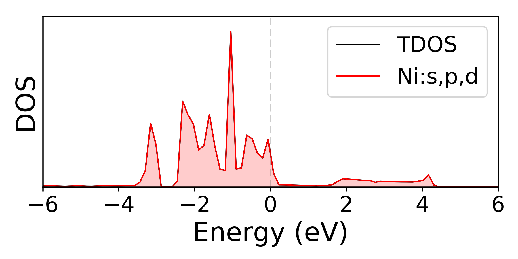
For DOS, the total DOS is always shown together with projected DOS (if computed). For /mcu/example/Ni, you can run

 import mcu
 mymcu = mcu.VASP()
 mymcu.plot_dos()

To customize the dos figure, one can modify some of these attributes.

 import mcu
 mymcu = mcu.VASP()

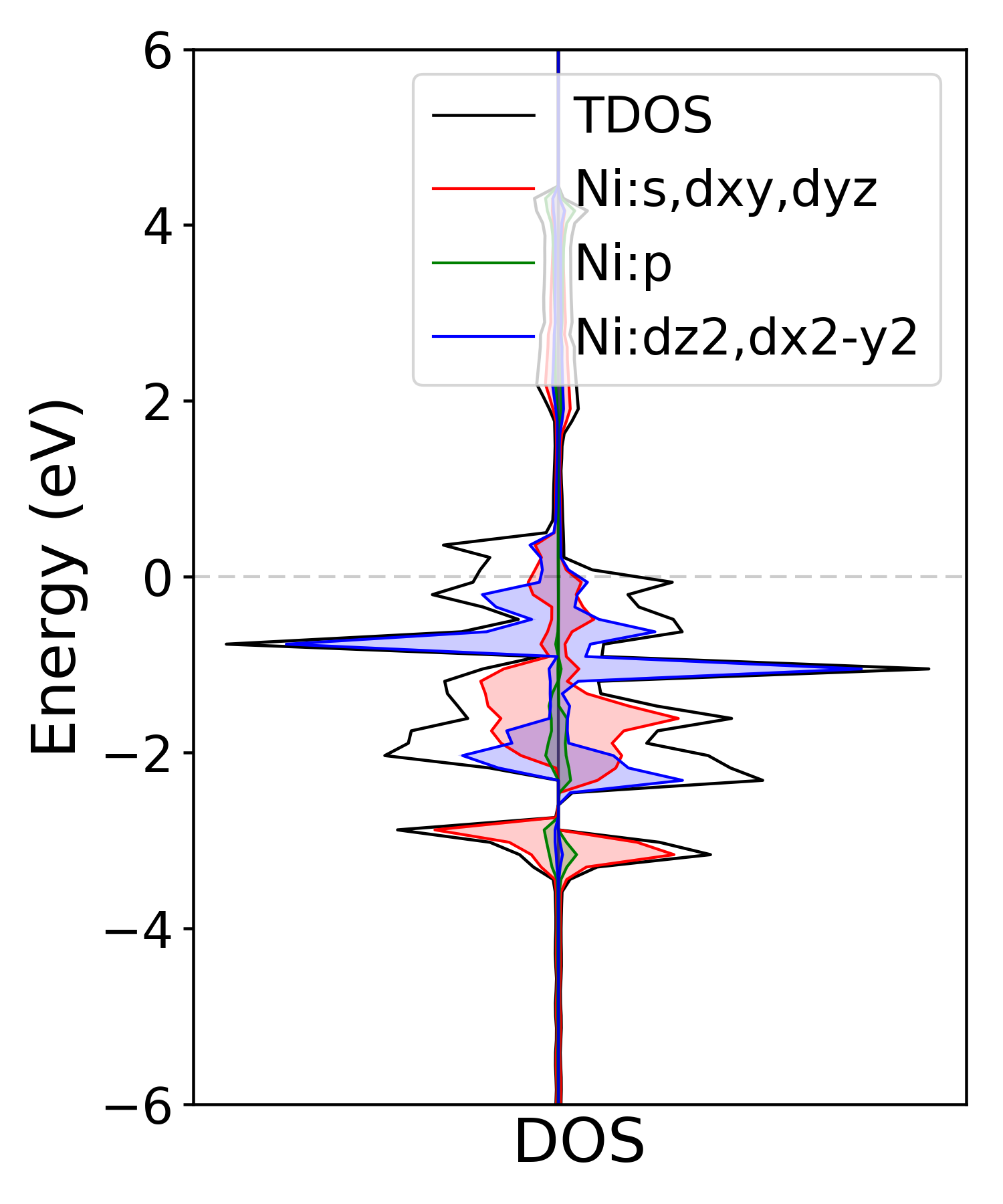
 # Style = 2 and spin = 'updown'
 mymcu.plot_dos(spin = 'updown', style = 2, lm = ['Ni:s,dxy,dyz','Ni:p','Ni:dz2,dx2-y2'], save=True, figname='Ni_updown', dpi=300)

You should get:

All parameters and their defaults of plot_dos function are given below.

Parameters¶

vasprunobject

Defaul: None
If multiple vasprun.xml files are used when defining a mcu object then user can pick of of those. By default, the first vasprun.xml in the list will be used

styleint

Default: 1
style = 1 (standard plot) or style = 2 (vertital plot)

efermifloat

Default: fermi level from vasprun.xml or OUTCAR
User can shift the Fermi level to a value

spinint

Default: 0
If ISPIN = 1: spin = 0
If ISPIN = 2: spin = 0 (Up spin) or 1 (Down spin). spin = ‘updown’ means plotting both alpha and beta electrons
For LSORBIT = True: spin = 0 (total m) or spin = 1 (mx) or spin = 2 (my) or spin = 3 (mz)

lmstr or a list of str

Default: DOS is projected on each atom.
Example: ‘Ni:s’ or [‘Ni:s’,’C:s,px,pz’]

colorlist

Default: None
By default, there is a list of random color codes in plot_pband functions can be used. It is not used if style = 3
User can provide a list of color they wish to use. For example, [‘r’,’#ffffff,’k’]. Just need to make sure the numbers of color code should match with the numbers of group of orbitals plotted. For example, lm =’spd’ then there should be a list of three color codes.
Hex color code can be found here here

legendlist of str

Defaul: None
A list of labels for different group of orbitals. For example, [‘Mo_s’,’S_p’]

loc :

Defaul: “upper right”
Location of legend
Possile loc value can be found here . Look for ‘Location String’ or ‘Location Code’

fillbool

Default: True
Whether to fill the area below the DOS curve.

alphafloat

Default: 0.2
Used to adjust the transparency of the marker

savebool

Default: False
True to save to an image

figsizetuple or list

Default: (6,6)
Size of image in inch

fignamestr

Default: ‘DOS’
Name of the image

elimlist

Default: [-6,6]
Limit range for energy axis in eV

yscalefloat

Default: 1.1
Used to zoom in and out the horizontal or DOS axis

fontsizeint

Default: 18
Font size

dpiint

Default: 600
Resolution of the image

formatstr

Default: ‘png’
Extension of the image

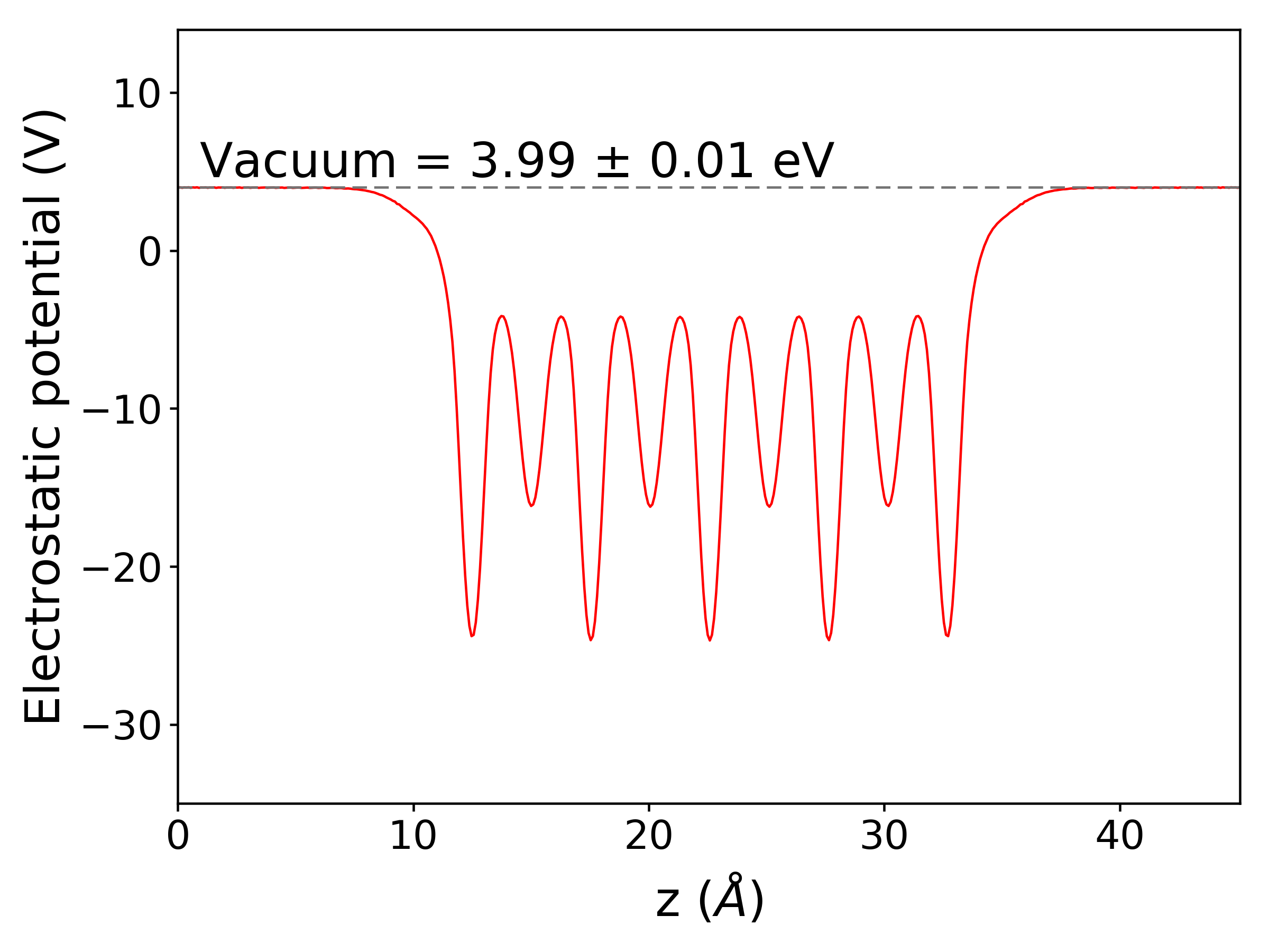
Work function and the electrostatic potential over a plane¶

The work function \(\Phi\) is defined as:

\[\Phi = - E_{VBM} = E_{Vacuum} - \epsilon_F\]

where \(\epsilon_F\) and \(E_{Vacuum}\) are the Fermi level and the electrostatic potential of vacuum, respectively. The \(E_{Vacuum}\) can be computed by simply constructing a slab model and adding LVTOT = .TRUE. to INCAR in VASP calculation. LOCPOT file , where the electrostatic potential is computed on the fine FFT-grid, will be generated as a result. The average over a plane perpendicular to an crystal axis can be computed and plotted via mcu.

You can run the below commands in the /mcu/example/InCuCl directory

import mcu
mymcu = mcu.LOCPOT()
mymcu.plot(axis='z', error=0.01)

You should get:

In case you want to get the electrostatic potential data and plot it yourself

import mcu
mymcu = mcu.LOCPOT()
pot = mymcu.get_2D_average(axis='z')                       # an 2 dimensional array [x,y] with x is the coordinates and y is the potential
e_vacuum = mymcu.get_2D_average(axis='z', error=0.01)      # to get E_vacuum

All parameters and their defaults of plot function are given below.

Parameters¶

axisstr

Default: ‘z’
The average of electrostatic potential is computed over a plane that is perpendicular to this axis

errorfloat

Default: 0.01
The electrostatic potential (pot) at the vacuum is computed by taking the average of all the pot in the window (pot - 2*error, maximum of pot)

colorlist

Default: [‘r’, ‘#737373’]
The color codes for the electrostatic potential and the vacuum marker

ylimlist

Default: None, automatic estimated
Limit range for energy axis in eV

savebool

Default: False
True to save to an image

figsizetuple or list

Default: (8,6)
Size of image in inch

fignamestr

Default: ‘elecpot’
Name of the image

fontsizeint

Default: 18
Font size

dpiint

Default: 600
Resolution of the image

formatstr

Default: ‘png’
Extension of the image